Decision Trees are Suboptimal!
The decision tree is one of the first classification algorithms taught in any machine learning course. It is easy to understand and gives a very interpretable output. Despite this, most people don't realise that all tree building algorithms (e.g. CART, ID3, C.45, MARS) are suboptimal.
Suboptimal in this context is not referring to how good or bad these classifiers perform on an arbitrary dataset (and it is likely that a decision tree will not give the best results for most real world datasets). Instead, we are going to explore how well a decision tree does the job that it is supposed to do - classifying a dataset by repeatedly splitting on the features. You will see that even if the dataset can be classified perfectly using a tree, it is very unlikely that a decision tree algorithm will find that optimal tree successfully.
This behaviour is a necessary compromise to allow decision trees to scale well to large datasets, and trying to actually find the optimal tree is a problem that quickly becomes unachievable as we start talking about even a modestly sized dataset. So whilst unavoidable in any practical application, it is worth being aware of these limitations in the algorithms and this post will expore this in some detail.
The dataset
In order to put decision trees to the test, we need to generate a dataset which we know can be solved by a tree. To start off with, we will generate a dataset where one class is sampled uniformly from the 2 blue sections below, and the other class is sampled from the yellow sections (while making sure there is at least one point in each of the 4 sections). This dataset can then definitely be split by the tree of depth 2, and cannot be split by a tree of depth 1.

For this dataset, an optimal decision tree should be able to split the data on the green dotted lines above, producing the following decision tree:

Initial results
Now we have defined our dataset, we can try to classify it using a CART decision tree. Note, there are no training/testing datasets here as we are just trying to see if the classifier can even fit to our dataset, without worrying about whether or not it overfits.
For this we will be using the DecisionTreeClassifier from python's scikit-learn, but the implementation should not make too much difference to the conclusions drawn - there will be a very similar story for every decision tree algorithm. If you would like to follow along with the code, click the 'Toggle Code' button at the top of the page.
After trying out the decision tree on a dataset with 10 points, this is what we get:

The decision tree took 3 splits to separate the data! This may come as a surprise considering how obvious it is to the human eye that this dataset can be split in just 2 splits. A deeper tree will do a worse job at generalizing to new unseen data, and this is evident in the figure above. The blue background shows all of the points which would have been given the blue class, and you can see that this area is much larger than the area used to create the blue points.
Was that a fluke?
After seeing this, your initial reaction may be that this dataset has been specifically crafted so that the decision tree does a poor job. To test this out, we can generate many datasets of various sizes, and see how many the decision tree manages to classify using an optimal (depth 2 in this case) tree. The results of that analysis are shown below:

From this plot we can see that for very small datasets the decision tree finds the optimal tree most of the time, which makes sense because there are only a few possible trees which can be built when there are very few points. However, as soon as we get beyond 20 or so points it becomes very unlikely that the decision tree algorithm will find the optimal tree.
So what is going on then?
The decision tree algorithm is greedy, and this is why it is falling short here. The datasets we are using are not particularly special, but they were chosen so that the best depth 1 tree does not produce the optimal depth 2 tree. This property is going to exist in pretty much every real world dataset to some extent, but our chosen data distribution highlights this shortcoming in an obvious way.
By plotting the decision boundaries at each depth of the decision tree, we can understand how the greedy algorithm came to generate a suboptimal tree.
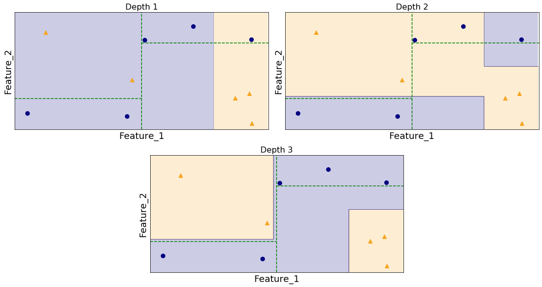
The decision tree starts by finding the best initial split of the data. It manages to find a split which has a LHS gini impurity of:
and a RHS gini impurity of:
leading to an average of \(0.409...\).
In comparison, the optimal depth 2 tree at depth 1 has an average gini impurity of \(0.5\).
A smaller gini impurity indicates a better split, with 0.5 being the worst possible value. So at the first level, the CART decision tree algorithm did a better job. In fact, by just looking at the first level of the eventual optimal tree, the impurity has not been improved at all and the dataset is just as unclassified as it would be if the classification was left to random chance.
However, by the second level the gini impurity of the decision tree algorithm drops to \(0.222...\) while the optimal tree has an impurity of 0 indicating a perfect split. By being greedy at the first level, the decision tree algorithm failed to find the best possible solution after two levels.
It takes until the third level for the decision tree to completely separate the datasets.
In fact, it is not too hard to find a dataset where a decision tree will generate a far deeper tree, such as the one below of depth 7!

The depth 7 tree manages to correctly classify all the data, but is clearly going to generalize poorly. For example, the unseen point \((1.75, -0.5)\) shown as a black cross will be misclassified as blue, when it clearly should be yellow. By comparing this decision tree at depth 2 to the optimal tree, we can see that restricting the tree depth will not give a better solution here.
Can we do better?
A way to potentially eleviate this problem is to use a random forest, which is a collection of decision trees trained on random subsets of the data.

A random forest of depth 2 trees still does a very poor job on the dataset, and there is a whole region in the upper left where it fails to identify the correct class. However, a random forest of depth 7 trees does a better job on the dataset and it is clear that the imperfections of each tree individually have been smoothed out by the forest. Although, it is interesting to note that the combination of 1000 decision trees of depth 7 has still failed to optimally split a dataset which can be split by a simple tree of depth 2!
The fact is that there are simply too many possible trees to check every single one for the best score. Granted, in this case it would be pretty easy to write something to check all depth 1 and depth 2 trees to find the best one, but that will not scale when the depth of the tree gets into double (or even triple) digits, and it will also not scale well as the dataset grows. Ultimately every algorithm has to find a balance between accuracy and speed, and being greedy is the compromise made by most (if not all) decision tree implementations. This should not stop you from using them as tree methods still have a great number of benefits, but it should help give you a better idea about how the algorithm works.